AdaptiveTimeScale.py--Easy dateticks for Matplotlib time-series plots

Introduction

Matplotlib is the python programming language's plotting library. It is extraordinarily sophisticated, capable of producing a huge variety of plot types, as a glance at its gallery page will demonstrate.

When plotting time-series data in matplotlib, an experienced user can set the labels of the axis ticks individually to have whatever format s/he desires, but this requires skill and effort.

There is an automated datetick-labelling functional called "autofmt_xdate()" built into matplotlib that works in many circumstances, but frequently the results are disappointing, as shown below.

The Problem

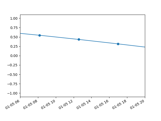
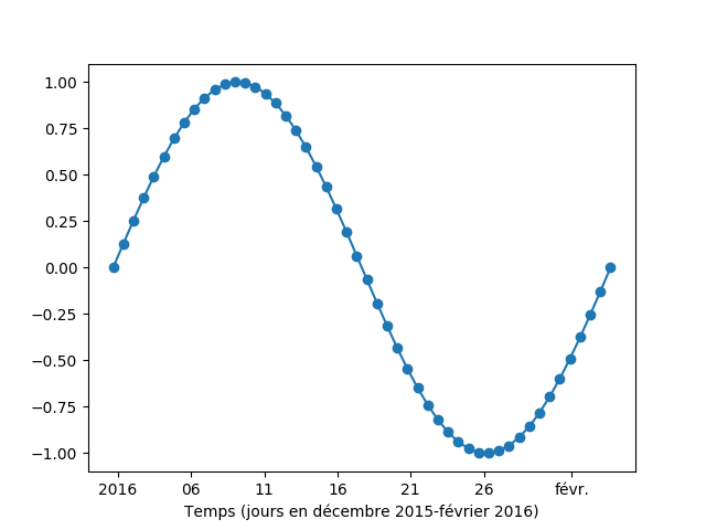
autofmt_xdate(), Matplotlib's automated datetick labelling function, puts all of its date and time information into every tick it generates. This can result in highly cluttered plots, as the year, month, and day values appear in every single tick, even when redundant.

Example 1: autofmt_xdate() clutters plots with redundant date information. All ten tick labels in this figure contain the exact same year and month value.

When the time limits of the plot are tight enough that hours, minutes, or seconds need to be shown, the situation is even worse. With so much information to cram into each tick label, autofmt_xdate() is forced to abbreviate some information and leave some information out, resulting in cryptic and ambiguous date/time strings.

Example 2: autofmt_xdate() creates ambiguous and cryptic tick labels when it runs out of space. What date and time does "01-05 08" correspond to?

The Solution

AdaptiveTimeScale puts as much redundant date and time information as possible into the axis label, rather than trying to include it in each individual tick. This saves enough space that dates and times do not need to be shortened in order to fit. The result is readable and unambiguous date tick labels.

Example 3: Plot produced using AdaptiveTimeScale. "January 2005" is information common to all five date ticks, so it is shown in the axis label.

Example 4: Plot produced using AdaptiveTimeScale. Here, the year, month, and day are shown in the axis label, leaving room for unambiguous and readable tick labels.

How to use AdaptiveTimeScale

AdaptiveTimeScale is easy to use. The following code is pretty much the same code you'd use to make a plot using autofmt_xdate(). The two lines specific to AdaptiveTimeScale have been highlighted, and the call to autofmt_xdate() has been removed.


import AdaptiveTimeScale
import matplotlib.pyplot as plt
import numpy as np
import datetime as dt
import matplotlib.dates as mdate
numPts = 50
startTime = dt.datetime(2005, 1, 1, 16, 0, 0, 0)
endTime = dt.datetime(2005, 1, 10, 16, 0, 0, 0)
x = [mdate.num2date(i) for i in np.linspace(mdate.date2num(startTime),mdate.date2num(endTime),numPts)]
y = [np.sin(i) for i in np.linspace(0,2*np.pi,numPts)]
fig, ax = plt.subplots() 
plt.plot(x,y,'o-')
fig.autofmt_xdate()
ax.set_xscale('adaptivetime')
plt.show()

Keyword arguments can be used to modify AdaptiveTimeScale's behaviour. Tick and axis labelling can be disabled entirely (doLabelTicks and doLabelAx); the maximum number of ticks can be increased or decreased from the default of 8 (maxTicks); and a time zone string can be appended to the axis label (timeZoneStr).

Example 5: Plot produced using AdaptiveTimeScale. Tick and axis labelling have been suppressed in the upper axes, the maximum number of ticks increased to 10, and the time zone string "UTC" has been appended to the axis label.


import AdaptiveTimeScale
import datetime as dt
import numpy as np
import matplotlib.pyplot as plt
y = np.array([440, 100, 200, 50, 400, 300, 60, 70, 80, 90])
timeDelta = dt.timedelta(days=1)
t0 = dt.datetime(2015, 12, 31, 16, 0, 0, 0)
t = [t0 + timeDelta * j for j in range(len(y))]
tlims = [np.min(t),np.max(t)]
fig = plt.figure()
ax1 = fig.add_subplot(2,1,1)
ax1.plot(t, y,'o-')
ax1.set_xlim([tlims[0],tlims[1]])
ax1.set_xscale('adaptivetime',doLabelTicks=False,doLabelAx=False,maxTicks=10)
ax1.set_ylabel('y')
ax2 = fig.add_subplot(2,1,2)
ax2.plot(t, y,'o-')
ax2.set_xlim([tlims[0],tlims[1]])
ax2.set_xscale('adaptivetime',timeZoneStr="UTC",maxTicks=10)
ax2.set_ylabel('y')
plt.show()

Internationalization and Customization

AdaptiveTimeScale can easily be converted to work with other languages by the addition of a custom "module" (python .py file) that overrides AdaptiveTimeScale's generate_axlabel() and generate_ticklabel() functions (this same method could be used to customize date and time formats in English).

Example 6: French-language plot produced using AdaptiveTimeScale, with custom versions of generate_axlabel() and generate_ticklabel() defined in a file called "my_custom_formats_french.py".


import AdaptiveTimeScale
import matplotlib.pyplot as plt
import numpy as np
import datetime as dt
import matplotlib.dates as mdate
numPts = 50
startTime = dt.datetime(2005, 1, 1, 16, 0, 0, 0)
endTime = dt.datetime(2005, 1, 10, 16, 0, 0, 0)
x = [mdate.num2date(i) for i in np.linspace(mdate.date2num(startTime),mdate.date2num(endTime),numPts)]
y = [np.sin(i) for i in np.linspace(0,2*np.pi,numPts)]
fig, ax = plt.subplots() 
plt.plot(x,y,'o-')
ax.set_xscale('adaptivetime',CustomModule='my_custom_formats_french')
plt.show()

AdaptiveTimeScale

Features

Introduction

The Problem

The Solution

How to use AdaptiveTimeScale

Internationalization and Customization

Where can I get AdaptiveTimeScale.py?

Contact us